Hypothesis Testing Continuous Outcome Matched Samples
Problem Statement
The sample dataset has placement test scores (out of 100 points) for four subject areas: English, Reading, Math, and Writing. Students in the sample completed all 4 placement tests when they enrolled in the university. Suppose we are particularly interested in the English and Math sections, and want to determine whether students tended to score higher on their English or Math test, on average. We could use a paired t test to test if there was a significant difference in the average of the two tests.
Before the Test
Variable English has a high of 101.95 and a low of 59.83, while variable Math has a high of 93.78 and a low of 35.32 (Analyze > Descriptive Statistics > Descriptives). The mean English score is much higher than the mean Math score (82.79 versus 65.47). Additionally, there were 409 cases with non-missing English scores, and 422 cases with non-missing Math scores, but only 398 cases with non-missing observations for both variables. (Recall that the sample dataset has 435 cases in all.)
Let's create a comparative boxplot of these variables to help visualize these numbers. Click Analyze > Descriptive Statistics > Explore. Add English and Math to the Dependents box; then, change the Display option to Plots. We'll also need to tell SPSS to put these two variables on the same chart. Click the Plots button, and in the Boxplots area, change the selection to Dependents Together. You can also uncheck Stem-and-leaf. Click Continue. Then click OK to run the procedure.
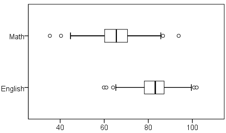
We can see from the boxplot that the center of the English scores is much higher than the center of the Math scores, and that there is slightly more spread in the Math scores than in the English scores. Both variables appear to be symmetrically distributed. It's quite possible that the paired samples t test could come back significant.
Running the Test
- Click Analyze > Compare Means > Paired-Samples T Test.
- Select the variable English and move it to the Variable1 slot in the Paired Variables box. Then select the variable Math and move it to the Variable2 slot in the Paired Variables box.
- Click OK.
Syntax
T-TEST PAIRS=English WITH Math (PAIRED) /CRITERIA=CI(.9500) /MISSING=ANALYSIS. Output
Tables
There are three tables: Paired Samples Statistics, Paired Samples Correlations, and Paired Samples Test. Paired Samples Statistics gives univariate descriptive statistics (mean, sample size, standard deviation, and standard error) for each variable entered. Notice that the sample size here is 398; this is because the paired t-test can only use cases that have non-missing values for both variables. Paired Samples Correlations shows the bivariate Pearson correlation coefficient (with a two-tailed test of significance) for each pair of variables entered. Paired Samples Test gives the hypothesis test results.
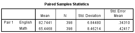
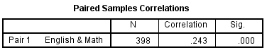
The Paired Samples Statistics output repeats what we examined before we ran the test. The Paired Samples Correlation table adds the information that English and Math scores are significantly positively correlated (r = .243).
Why does SPSS report the correlation between the two variables when you run a Paired t Test? Although our primary interest when we run a Paired t Test is finding out if the means of the two variables are significantly different, it's also important to consider how strongly the two variables are associated with one another, especially when the variables being compared are pre-test/post-test measures. For more information about correlation, check out the Pearson Correlation tutorial.

Reading from left to right:
- First column: The pair of variables being tested, and the order the subtraction was carried out. (If you have specified more than one variable pair, this table will have multiple rows.)
- Mean: The average difference between the two variables.
- Standard deviation: The standard deviation of the difference scores.
- Standard error mean: The standard error (standard deviation divided by the square root of the sample size). Used in computing both the test statistic and the upper and lower bounds of the confidence interval.
- t: The test statistic (denoted t) for the paired T test.
- df: The degrees of freedom for this test.
- Sig. (2-tailed): The p-value corresponding to the given test statistic t with degrees of freedom df.
Decision and Conclusions
From the results, we can say that:
- English and Math scores were weakly and positively correlated (r = 0.243, p < 0.001).
- There was a significant average difference between English and Math scores (t 397 = 36.313, p < 0.001).
- On average, English scores were 17.3 points higher than Math scores (95% CI [16.36, 18.23]).
nankervisidel1939.blogspot.com
Source: https://libguides.library.kent.edu/spss/pairedsamplesttest